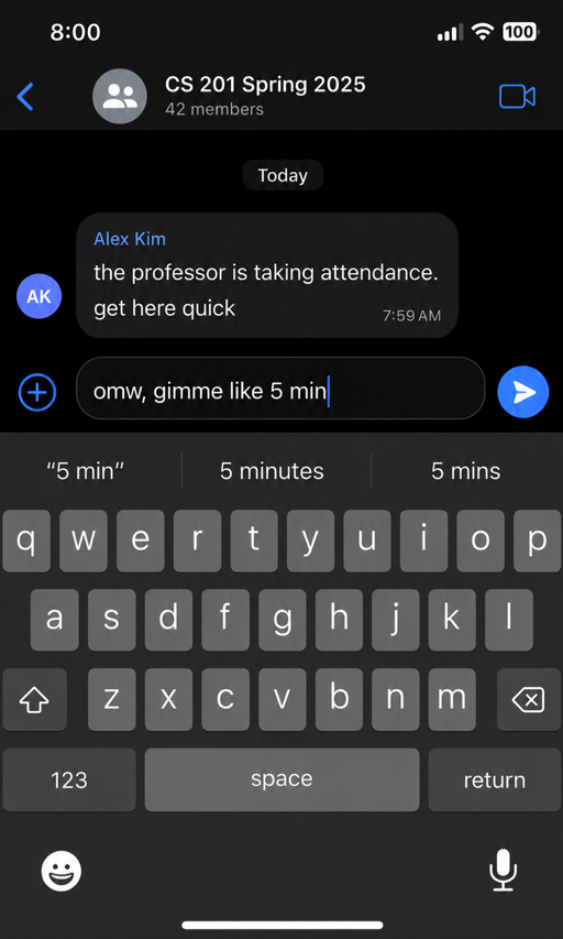
it's 8am. you just dressed up and you're getting ready to leave for class. on your class group chat, someone texts "the professor is taking attendance. get here quick" as you are throwing your bag over your shoulder, you start to type 'omw, gimme like 5 min—' and your keyboard's already finished half your sentence before you have.

anything unusual there? nah.

it's normal life for people who use phones. we type some letters in a word and the word we need show up in the suggestion box. in some cases, the phrase even shows up. what most folks don't know is what's responsible for that is the autocomplete system that's a part of your keyboard. it predicts the word thanks to a lot of computational work going on in the background

this piece is meant to introduce you to a good overview of the technology behind autocomplete, how it works under the hood and for the techy guys, we'll implement a very simple, but really really representative autocomplete system

alright, let's dive right into it!

history of autocomplete

i am not the biggest history buff but i believe that knowing the lore behind how something originated helps you appreciate it better and in some cases, maybe understand it more. in this particular case, it also reinforces the truth that most of the best things we use today came due to someone's necessity.

In the 1950s, a lot of Chinese engineers and researchers had a problem that was really really driving everyone crazy. If you've ever seen Chinese characters before, you'll realize that typing them on a normal keyboard isn't exactly the easiest job. thank God for English because it allows us to get away with just 26 letters. the Chinese have tougher luck though. as of 2025, over 100,000 Chinese characters have been documented, although only a few thousand are used regularly. regardless, that's… a lot.

so typing in Chinese was a hard thing for them. however, for every problem, there's most likely a solution (unless you're Ronaldo trying to win a World Cup). so people started asking a very engineering-like question: "surely there has to be a better way than pressing a million keys every time I want to write something."

the key insight was simple: the relationship between a character and the way it's written doesn't randomly change. if we can encode those characters and use them to build a large dictionary of possibilities, whenever someone types, we can narrow them down. this way, the computer can do most of the hard work instead of the human. classic human thinking — give the hardwork to the machine!

that idea began decades of research into Chinese input methods and predictive typing. autocomplete was the work of many people over many years, and there was never a singular moment of victory so to say. but those efforts became one of the earliest and strongest motivations for the predictive text systems we now take for granted.

so yes, wherever those researchers are, they deserve a little nod of appreciation. they were just trying to make typing less painful for themselves. the rest of us ended up getting autocomplete.

side note: you can actually solve problems as well. instead of complaining about how things are, think, innovate. let your frustration at broken systems or technologies drive you to proffer solutions to them. if you do it well enough, 70 years from now, one kid will be writing about you.

the how of autocomplete

autocomplete is really advanced. it's now a beautiful & intricate piece of technology and trying to fully explain how current systems work down to first principles would take up months of learning. but as anyone who codes regularly knows, the principles behind most things rarely changes. all we do is build on it to make it better & faster while also allowing it to accommodate more nuances. this applies to autocomplete. so what we'll do is go back to how it started and the initial framework.

it's technically impossible for us to explain the how of autocomplete if we don't go back in time to 1912. there, we see a mathematician called Axel Thue who wrote a paper titled "Über die gegenseitige Lage gleicher Teile gewisser Zeichenreihen". that's German for "On the Mutual Position of Equal Parts of Certain Strings of Symbols". in his paper, he abstractly described a structure that would be used to hold subsequences of strings. this concept was purely abstract and more mathematical than it was computational — infact, computers didn't even exist then. talk about being ahead of time lol.

it wasn't until computers came that Thue's idea became actually useful.

how did thue's idea become useful?

everything we do on a computer is done on its memory, so the speed of retrieving what is in which part of memory has always been very important. what was stored on a computer then was called a record.

the initial method used for accessing records was the sequential method — you put everything in a memory block in sequence, and when you need a particular record, you go over it one by one until you get what you want. the more records you have, the slower it gets.

innovation led to the index method: store an index for each record, and the index points to the record's exact location in memory. much more efficient compared to sequential, but searching for the index itself can get slower as records get bigger.

then came the "bucket" method: we use a function to generate a number for a record, and if that block in memory is unoccupied, the record goes there. if it's occupied, you find the closest empty space and note the difference.

these methods weren't bad but they wanted something optimized for words and language.

the trie: a structure built for words

so a computer scientist at that time, Rene De La Briandais, came up with a new approach that was faster and much suited to words.

Rene proposed that instead of us storing the name of the records and almost rummaging through memory anytime we needed them, why don't we store them in a pattern where we store the first letters of all the names of the record each.

let's imagine we have 7 words we want to store (bat, ball, bank, band, cat, car, care). instead of just storing them all at once, we create an array with all the first letters.

so [b, c].

wait, no repeats even though multiple words start with b or c? nope. that's the trick there. our array will only contain one instance of the first letters. so they only appear once.

where are the remaining letters? well, for each letter in that array we just created, we create a new separate box. in that box, we store the second letters. so our second box for b is [a] (bat, ball, bank, band all share "ba") and our second box for c is [a] (cat, car, care all share "ca"). we then continue repeating this until we reach the end of our record names — that's how "ba" eventually forks into t / l / n for bat/ball/band-bank, and "ca" forks into t / r for cat/car(e).

you can't really get the idea of this until you see it in a tree like structure.

graph TD
    root(( ))
    root --> B[b]
    B --> BA[a]
    BA --> BAT((t · bat))
    BA --> BAL[l]
    BAL --> BALL((l · ball))
    BA --> BAN[n]
    BAN --> BANK((k · bank))
    BAN --> BAND((d · band))
    root --> C[c]
    C --> CA[a]
    CA --> CAT((t · cat))
    CA --> CAR((r · car))
    CAR --> CARE((e · care))

do you see that? do you see the beauty of computational genius? look at it again and just marvel.

how is this more efficient?

to truly understand the beauty of this, you have to understand that before, when looking for a word, what we had to do was to check each and every word until we reached our desired word. so if we had an array of 10000 words, we have to check every single one in the worst case scenario.

in Rene's method, let's assume that 100,000 words are evenly distributed. so with 26 possible starting alphabets, add 10 possible numbers and some special characters to just make it 40. if we divide 100,000 words, we have around 250 words per each letter. so if we search for any word, we just have to check our array for if the first letter exists. it definitely does, but here's the good part — it leads us to completely eliminate 39 other entire letters and thereby completely remove their parts from our search. so we just have to search 250 words. we have completely eliminated 99,750 words.

we go down and we now again have 40 possible second letter combinations, each of them will have just 7 words each after them. you see how we just keep reducing our search pool drastically? that drastic reduction of the search pool is exactly what makes this structure optimized for word search. for each word we have, we go down a particular node and this way, we can ignore other nodes.

the example i gave is slightly improbable to be honest. all the words you want to store will most likely not be distributed evenly among the alphabets. however, the node traversal logic still applies.

that structure was independently built again by another scientist Edward Fredkin in 1960, and he called it "trie". he got the name from the middle syllable of retrieval. it's pronounced "TRY" by the way—

the computing world owes Rene & Edward a big one because that structure was perfect for autocomplete. if you think about it, it's so freaking optimized for it. when you type a, all we have to do is to look at the words we have under the "a" tree. if you add 'p', we move to the p branch under a. the more words you type, the more accurate suggestions we can give because the lesser branches we have. this explains why the more letters you type in autocomplete, the more accurate we are to getting the exact word you want!

bingo!

building a trie in python

now for the fun technical part. we are going to implement a trie in python! we'll add a couple of functions for searching as well. for non technical folks, you can skip the code and just jump to the next one.

first, we have the building block. every node in the trie holds three things: the children that can branch off it, a flag for whether a complete word ends there, and the finished word itself. the finished word is an empty string for allnodes except the one which signifies the end of a word.

import re

class TrieNode:
    def __init__(self):
        self.children = {}   # an empty dictionary to store each letter under the node
        self.is_end = False  # a boolean to indicate if we've reached the end of a word
        self.word = ""       # a string to store the words at each stage

next, the trie itself. intially, it starts as nothing but an empty root node. to add a word, we walk through the word letter by letter from the root and create a node wherever a letter doesn't exist yet. once we run out of letters, we use the flag in the last node to signify that and add the word to the node as well.

class Trie:
    def __init__(self):
        self.root = TrieNode()

    def add_word(self, word: str):
        curr = self.root
        for c in word:
            if c not in curr.children:
                curr.children[c] = TrieNode()
            curr = curr.children[c]
        curr.is_end = True
        curr.word = word

if we're adding words one at a time, that would take time. we want to just take a text file full of words and add it to our trie. so we added a small helper on the same class that reads an entire file, cleans it up, and drops every unique word into the trie.

    def preprocess_and_load_file(self, filepath: str, encoding: str = "latin-1"):
        """Reads a file, cleans it, splits it into words, and adds them to the Trie."""
        with open(filepath, "r", encoding=encoding) as file:
            text = file.read()
            text = text.lower()
            text = re.sub(r'[^a-z0-9\s]', '', text)
        words = text.split()
        unique_words = set(words)
        for word in unique_words:
            self.add_word(word)

that covers putting words in. now how do we get get them back out? once we've walked down to a node, we want every complete word sitting underneath it. the algorithm for doing this is called a depth first search: if the current node ends a word, save it, then dive into each of its children.

    def dfs(self, curr: TrieNode, res: list):
        if curr.is_end:
            res.append(curr.word)
        for child in curr.children.values():
            self.dfs(child, res)

and finally the search itself. we follow the typed prefix down the trie one letter at a time. if a letter isn't there, the prefix doesn't exist and we return an empty list. otherwise we hand the node we stopped on to dfs, which gathers every word below it.

    def search_word(self, pref: str) -> list:
        res = []
        curr = self.root
        for c in pref:
            if c in curr.children:
                curr = curr.children[c]
            else:
                return res  # Prefix not found
        self.dfs(curr, res)
        return res

the trie's blind spot

so the using the trie was pretty much how autocomplete worked for a while, and to be honest, it can do a good job on its own. the more letters the person types, the closer we get to the correct word.

but get your eyes off this screen for a bit and just think of this: "what's wrong with this current setup?"

there's a very great flaw that makes this setup alone just not good enough, especially for conversations and more nuanced things.

the biggest flaw in just using the trie alone is lack of context. let's assume someone is writing a sentence. the sentence they want to write is "i withdrew cash from the bank". assume they have typed out "ba" and we want to use the trie to get the possible words. as we can see in the code, our search function will perform a thorough search for all words that begin with "ba". the english dictionary is so large and full of words with "ba" and so we would end up with a lot. but we can't show them all to the user, can we? we have to pick maybe three to five. but, what's the criteria for picking one over the other? we don't have any.

in the absence of a law, everything is right. so we could end up showing them words like "banana", "bay", "banger", when the actual word they need is so obviously "bank".

i mean there's a probability we show them that word but there's a much larger chance we don't.

using the trie alone means we just leave things to chance and in computation, we don't do none of that. we have to guide the computer on what to do so we can predict its results and ensure they are as good as they can be.

making autocomplete smarter

so a bunch of things were added to make a trie much better and effective.

frequency weighting

the first was frequency weighing. this is really self-explanatory tbh. it's just like the name sounds.

what they did was to assign a probability to each word in the trie based on a big corpus. corpus just means a lot of documents. so they ran through a big corpus and then they count all the words. so the frequency weight of each word in it just becomes the number of times the word appeared divided by the total number of words in the corpus. as you might guess, this leads to a bias for repetitive words — words like "the", "and", "or", "of" and others get recommended very often.

in a way, this approach isn't wrong when you consider the fact that the main goal of autocomplete is to reduce the number of times you have to type repetitive words. frequency weighting does that pretty well. if you type "o", of and or show up almost instantly. with frequency weighing, they got better results for repetitive words.

but think about it — does this solve our problem of lack of context? no, it doesn't. we'll still have words showing up that are almost useless to what we are currently typing. just because a word frequently shows up doesn't mean it's useful to our context.

how do we give computers context?

better still, how can we give them that intuition to know that when someone says "I withdrew cash from the b__", the right word should most likely be bank. you know it because you have that intuition developed. by default, computers don't.

this question has been solved in a whole lot of ways. a lot of technology has been created to solve it and most of them are very very big with tons of complex things.

a solution that answered this question and many other questions is known as language models. what's a language model? just think of it as a system that has been trained to predict text. given a particular text (in more technical terms, we call this a token), a language model can predict the next text based on a series of calculations from pre-training data. language models are really broad and trust me, talking about them is a blog post of its own. infact, what we know as AI today is a broad class of language models known as large language models.

however, for the sake of this learning, we'll talk about a type of large language model that's more fundamental but can really improve the results of our current autocomplete system.

this language model is an n-gram model.

don't panic. it sounded weird and took a while for me to really grasp as well but once you do, n-gram models are one of the most intuitive language models out there. though they aren't in use as much, it's still a really good building block for understanding how language models work.

quick disclaimer: language models and large language models weren't developed solely for autocomplete. they are technologies that found an application in autocomplete.

n-gram models

"my dad withdrew cash from the b__"

how do you know that the right word in that place is bank?

i would say you did a lot of fill in the gaps questions when you were young but a better answer would be because you have read and used enough of the English vocabulary to know that money is withdrawn from a bank. you are smart, don't get me wrong, but if you have not seen a word being used before in a particular context, the chances you can fill in the gaps for it are almost zero.

yeah, i know someone doesn't believe me.

well, complete the sentence;

"je mange riz et d_____"

"but it's a different language".

yeah, if you are so smart and all knowing in regards to words, you would know it.

give this to a french speaking person though and they'll tell you "hmm, there's a high chance what comes next is du pain". just like how you've seen enough of English vocabulary and studied it well enough to be able to fill in the gaps, they've studied french enough.

what does this tell us? understanding or predicting the next word in a sentence isn't an inherent trait. it's something that's trained by consistent exposure.

so when you saw that question on withdrawing money, what your brain subconsciously does is to think of all the times it's seen the word withdrawn and then, it thinks of the words that it's seen after it. you can withdraw love. you can withdraw pretty much anything. but then your brain says "wait a minute, we have cash. that's money" — so it creates a probability of places where money can be withdrawn. bag is possible in the sense that you can take out money from it. but then it says "it's most definitely bank. i've seen more situations where withdraw cash is used with bank than i have of bag".

if you understood that last paragraph, congrats, you understand n-grams — and dare i say, you actually have a solid grasp of how chatgpt works.

quick sidedive: what chatgpt really does is predict word by word. so when you ask it a question, it firstly predicts a token, then predicts the next and the next and the next and the next. which is why you see chatgpt streaming the words for you one by one. how it predicts the next token is very advanced. it uses smth called a transformer architecture that allows it to actually have the context of basically the entire sentence. talking about transformers would be a rabbit hole for this, but yeah, it's really just predicting the next token continuously.

back to n-grams!

like i said, that idea of "i have seen more of this instance than that instance" is exactly what n-grams are. the question then becomes how do we give computers that.

we do that by exposing it to a large set of text or corpus. this large set of data is called training data. what we do is go through the training data and then tell the computer "hey, we've gone through a very big big corpus of text and we saw that the word 'bank' comes after withdraw this number of times." we basically give the computer a probability.

i'll use a group of sentences to explain how we give the computers that probability.

"The cat sat on the mat." "The cat ate the fish." "The dog chased the cat."

the word "the" occurs 6 times. to get the probability of the next possible word that could follow it — in 3 of the 6 times we see "the", it's followed by "cat" in this text. so the probability of the next word after "the" being "cat" is $\tfrac{3}{6}$.

the other words, "dog", "mat", "fish" all occur once. so probability of dog following the is $\tfrac{1}{6}$. the same is for mat and fish.

to write this in probability terms, we can say;

that's how we would do it for "the". according to the chain rule of probability, what we would do for subsequent words is to multiply all the probabilities of the words before it.

so for the word fish at the end of the sentence, our probability would look smth like

that's how the probability would look like. however, if we keep on doing this, especially for long long sentences, we would have such a large number of things to multiply with. this might work for short sentences but for long sentences, we stand a chance of seeing zero.

probability already is between 0 & 1. the more we multiply numbers between 0 and 1, the closer we get to zero — and more importantly, when we are trying to predict a particular word, the longer the subsequence, the greater the chance that particular subsequence doesn't exist in our corpus at all. this means we stand a chance of having smth that's zero anyways, which would then terminate the entire thing to zero.

this current setup is computationally expensive (calculating all that will take more and more time as the sentences increases) and also mathematically improbable (we have a chance of never having that particular sequence in our entire training dataset).

the markov assumption

well, as we have seen, when the world is faced with great troubles and it seems like all hope is lost, one knight in shining armor always rises up to save the day. our knight for this time is called Andrey Markov. Markov wasn't exactly trying to solve this exact problem — infact, he died in 1922, long before this became a computing problem. but before he died, he made an assumption that eventually became known as the Markov assumption: an occurrence is independent of all previous occurrences before it. a better way to call it is memorylessness — smth doesn't have any memory of what happened before it, so all we have to be concerned about is its current state.

if you've ever heard of the gambler's fallacy, this rings a bell. the gambler's fallacy is the idea that after a run of the same outcome, the opposite is "due" to even things out — if smth has a 50% chance and you've seen 10 in a row, the fallacy assumes the next 10 should lean the other way. but as Markov's assumption shows, each occurrence is independent of previous ones. every new attempt is 50-50 again.

anyways!

how does this apply to n-gram models. well, our idea before was to use chain rule with all the previous probability.

so:

well, what the Markov assumption helps us do is we can cut this down and just say

shorter formula and probably more intuitive. instead of us trying to worry about all previous words before this current word, let's worry more about the n number of words before it — and that's why we have n-gram models.

the value of n is now dependent on you. if you want, you can choose to be concerned with only the word before it — that's called a bigram. you can say the last 2 words — that's a trigram. you can be lazy like me and just say, let's just guess — that's a unigram.

just like that, we've broken down how n-grams work.

building a bigram model

for technical folks, we'll build one in the next section. let's build a bigram — more common and easier to understand. for non technical people, you can skip, but in the next section, we'll use the model we build to get better autocomplete results.

a bigram model is really just a big tally of which word tends to follow which. so at its core, it's a map from a word to a counter of everything that's ever come right after it.

import re
import random
from collections import defaultdict, Counter

class BigramLanguageModel:
    def __init__(self):
        # Maps: current_word -> { next_word: count }
        self.bigram_counts = defaultdict(Counter)

before we can count anything, we need to turn raw text into clean, lowercased tokens. this little helper strips out punctuation and splits the text into a list of words.

    def _preprocess(self, text: str) -> list[str]:
        """Internal helper to clean and tokenize text."""
        text = text.lower()
        text = re.sub(r'[^a-z0-9\s]', '', text)
        return text.split()

training a bigram model is just walking through those tokens two at a time. for every word, we bump the count of the word that came right after it. when you do that across a whole book, you've got a real sense of what usually follows what.

    def train_from_file(self, filepath: str, encoding: str = "latin-1"):
        """Reads a file, preprocesses it, and builds the bigram frequency map."""
        with open(filepath, "r", encoding=encoding) as file:
            tokens = self._preprocess(file.read())
        # Build the bigram pairs
        for i in range(len(tokens) - 1):
            current_word = tokens[i]
            next_word = tokens[i + 1]
            self.bigram_counts[current_word][next_word] += 1

counts are just frequencies. but we dont want frequencies. what we want are the probabilities. so, to get the chance of each next word, we divide its count by the total number of words we've seen following the current one. and once we have that distribution, getting out the top n is just a sort.

    def get_probabilities(self, word: str) -> dict[str, float]:
        """Calculates the conditional probability distribution for a given word."""
        word_counts = self.bigram_counts.get(word.lower())
        if not word_counts:
            return {}
        total = sum(word_counts.values())
        return {next_word: count / total for next_word, count in word_counts.items()}

    def predict_next_top_n(self, word: str, n: int = 5) -> list[tuple[str, float]]:
        """Returns the top N most likely next words with their probabilities."""
        probs = self.get_probabilities(word)
        return sorted(probs.items(), key=lambda x: x[1], reverse=True)[:n]

for fun, we can also let the model ramble. starting from a seed word, we keep predicting the next word and feeding it back in. we have two flavors here: greedy always grabs the single most likely word, while weighted sampling rolls the dice using the actual probabilities: this reads a lot less robotic.

    def generate_text(self, start_word: str, length: int = 10, deterministic: bool = False) -> str:
        """Generates a sequence of words starting from a seed word."""
        current = start_word.lower()
        result = [current]
        for _ in range(length):
            probs = self.get_probabilities(current)
            if not probs:
                break
            if deterministic:
                # Always pick the absolute highest probability word (Greedy search)
                current = max(probs, key=probs.get)
            else:
                # Weighted random sampling based on the actual corpus distribution!
                words = list(probs.keys())
                weights = list(probs.values())
                current = random.choices(words, weights=weights)[0]
            result.append(current)
        return " ".join(result)

as you can see, we now have our bigram model working. i trained the bigram model on The Adventures of Sherlock Holmes by Arthur Conan Doyle. it's a big book and it definitely has enough varieties of sentence to serve our purpose. for emphasis, this counts as a really really small model: a good one would be trained on hundreds of those kinds of books. do remember, we're just learning the foundational principles.

so now, let's make some predictions.

bigram_model = BigramLanguageModel()
bigram_model.train_from_file("sherlock_holmes.txt")

# what's most likely to follow "the"?
print(bigram_model.predict_next_top_n("the", n=5))
# [('door', 0.014627430734813285), ('matter', 0.01428325589399415), ('other', 0.013766993632765444), ('house', 0.010841507485802787), ('room', 0.010497332644983651)]

# let's generate a short sequence, greedy style
print(bigram_model.generate_text("the", length=10, deterministic=True))
# "the door and i have been a little more than the"

# and now with weighted random sampling instead
print(bigram_model.generate_text("the", length=10, deterministic=False))
# "the care about to the small table waiting for it was"

(your exact output will always differ depending on the corpus you train on: these are illustrative of what the model spits out, not guaranteed values)

as we can see, using our text to generate the stuff gave us a random response. very very random one to be honest. but that's just the thing about n-gram models, they can give us very very random results. our training data was also very small, so that affected the results we got. the point is you can now see why n-grams aren't as good as the models we know today — so n-grams on their own aren't strong enough. but what if we add our trie structure. as the person types, we get all possible words we have in our trie and then we run them through our n-gram to get the one with the highest probabilities. those are the ones we display.

combining the trie and the bigram

here's the pipeline visually — trie narrows the world, bigram ranks what's left:

flowchart LR
    A["typed so far\nprevious: the\nprefix: ba"] --> B["trie\nsearch_word('ba')"]
    B --> C["candidates\nback, banker, bank,\nband, bar, banana…"]
    C --> D["bigram\nP(word | the)"]
    D --> E["ranked top-n\n1. back\n2. banker\n3. bank"]

think of it like a night out at a club or something. the trie is the bouncer at the door. doesn't care who you are, doesn't care about vibes, just checks one thing: does your name start with "ba"? if it doesn't, you're not getting past the rope. simple, fast, no context needed. the bigram is more like the bartender inside. by the time you're in, the bouncer's already done their job and now the bartender's looking at everyone who made it through and going "okay, who just walked up to me, and who's actually likely to be next based on who i've been serving all night." context matters here unlike at the door. neither one can do the other's job tbh. the bouncer isn't picking your drink order and the bartender definitely isn't checking IDs for the entire city. but when you put them together, you go from "every single word starting with ba in the english language" down to like 3-5 suggestions that actually make sense, all in the time it takes you to blink.

so now, let's try it again.

def autocomplete(trie: Trie, bigram_model: BigramLanguageModel, previous_word: str, prefix: str, top_n: int = 5):
    """Combines the trie and the bigram model: get every word that matches the prefix,
    then rank them by how likely they are to follow the previous word."""
    candidates = trie.search_word(prefix)
    if not candidates:
        return []

    probs = bigram_model.get_probabilities(previous_word)

    # score each trie candidate by its bigram probability (0 if the model has never seen it)
    scored = [(word, probs.get(word, 0)) for word in candidates]
    scored.sort(key=lambda x: x[1], reverse=True)

    return scored[:top_n]


# example: "i withdrew cash from the ba__"
results = autocomplete(my_trie, bigram_model, previous_word="the", prefix="ba")
print(results)
# [('back', 0.0017208742040956805), ('banker', 0.0015487867836861124), ('bank', 0.0013766993632765446), ('band', 0.0005162622612287042), ('bar', 0.00034417484081913615)]

you see how we can easily narrow down our choices to a more probable outcome when we combine the two? yes, the top choice "back" isnt right but we have "bank"and "banker" in our top 3 because they are both valid completions of "ba" and a word the model has actually seen follow "the". so any word starting with "ba" doesn't just get an equal shot.

voila!

before we wrap up, i added soemthing fun! if you want the whole story in one place, this is a clickable walkthrough of how autocomplete moved, era by era. hit the steps (or prev / next) to see it grow from "too many characters" to the keyboard in your pocket:

it's been a long long read so far but for your time, you now have a good grasp of one of the most used technologies in the world today. we've dived into the historical parts, the technicalities and even built a mini working version.

yayyy. we did it!

modern autocomplete system

what we built today is representative of how autocomplete systems work today but it's not the all in all. infact, there is so much more advanced technology that's being improved upon daily to ensure that the predictions are as accurate as they can possibly be.

a good one we can dive a little into is the personalization of autocomplete.

as i am pretty sure you've noticed, your keyboard can complete phrases or specific words you use often even if it's not in the English language. so if i use "Howard" very often, the chances it will show me "Howard" when i type "Ho" is higher than someone who doesn't use it. this is especially more noticed for those of us with non English names. your keyboard knows your name and if you type your address frequently, it can help you type it out once you type the first 2-3 letters in it and confirm the first word. this is achieved by a combination of multiple things. one of them is by storing the frequent words you personally use. most times, this storage is on your device so don't worry about your details being kept or smth lol. frequency weighing is also used to determine words that occur frequently per user and more importantly, the advanced models being used today are also trained on your repeated words. a lot goes on in that small phone of yours ngl

if you are technical, you can and should dive more into this topic. you should learn more about advanced large language models, neural nets, transformer architecture and more. they will definitely come in handy.

but if you are just a non-technical person who happens to just enjoy understanding how things work, you really have a good grasp. The next time your keyboard finishes your sentence before you do, you'll know there's decades of computer science quietly working behind that tiny suggestion bar.

if you wish, you can stop here. if you however wish to know more, i am happy to have helped you lay the foundation and i must here release you to greater enlightenment.

i sincerely hope this was informative for everyone. i myself was pretty clueless on this when i started, so i had to read a ton of papers, watch youtube videos and go through multiple ai summaries to be able to produce this. i hope you enjoyed reading it as much as i enjoyed writing it.

references

these are the papers, books, and resources i leaned on while writing this. the people behind them did the real work. you should read them if you want to go deeper.

1. Axel Thue. "Über die gegenseitige Lage gleicher Teile gewisser Zeichenreihen" ("On the Mutual Position of Equal Parts of Certain Strings of Symbols"), 1912.
2. Rene de la Briandais. "File Searching Using Variable Length Keys." Proceedings of the Western Joint Computer Conference (1959), p. 295 — the original trie.
3. Edward Fredkin. "Trie Memory." Communications of the ACM, 3(9):490–499 (September 1960). First circulated as an informal BBN memorandum, Cambridge, Mass., January 23, 1959.
4. Daniel Jurafsky & James H. Martin. Speech and Language Processing (3rd edition draft, January 6, 2026). web.stanford.edu/~jurafsky/slp3
5. "Natural Language Processing." Higher School of Economics, National Research University.
6. Wikipedia. "Autocomplete." en.wikipedia.org/wiki/Autocomplete